Simulation-Efficient Implicit Inference with Differentiable Simulators
Ecole thématique du CNRS - Future Cosmology
April 28, IESC Cargese, France
Justine Zeghal, François Lanusse, Alexandre Boucaud, Denise Lanzieri


Context
$ \underbrace{p(\theta|x_0)}_{\text{posterior}}$ $\propto$ $ \underbrace{p(x_0|\theta)}_{\text{likelihood}}$ $ \underbrace{p(\theta)}_{\text{prior}}$
$\to$ Full-Field Inference
Pros:
Information beyond Gaussian signal
Cons:
Need large number of simulations
Computationnally expensive (HMC)
Our goal: doing Implicit Inference with a minimum number of simulations.
Differentiable Mass Maps simulator
We developped a Differentiable LogNormal Mass Maps simulator
with 5 tomographic bins
and 6 cosmological parameters to infer.
sbi_lens package developped with Denise Lanzieri
For our studies, we used LSST Year 10 configuration.
Why LogNormal?
- Information beyond Gaussian signal
- Realistic enough for our purpose
- Fast
Implicit Inference
With infinite number of simulations, our Implicit Inference contours are as good as the Full Field contours obtained through HMC
But now, how can we reduce this number of simulations?
$\to$ by using the gradients $\nabla_{\theta} \log p(\theta|x)$ (also known as the score) from our differentiable simulator
Gradient constraining power


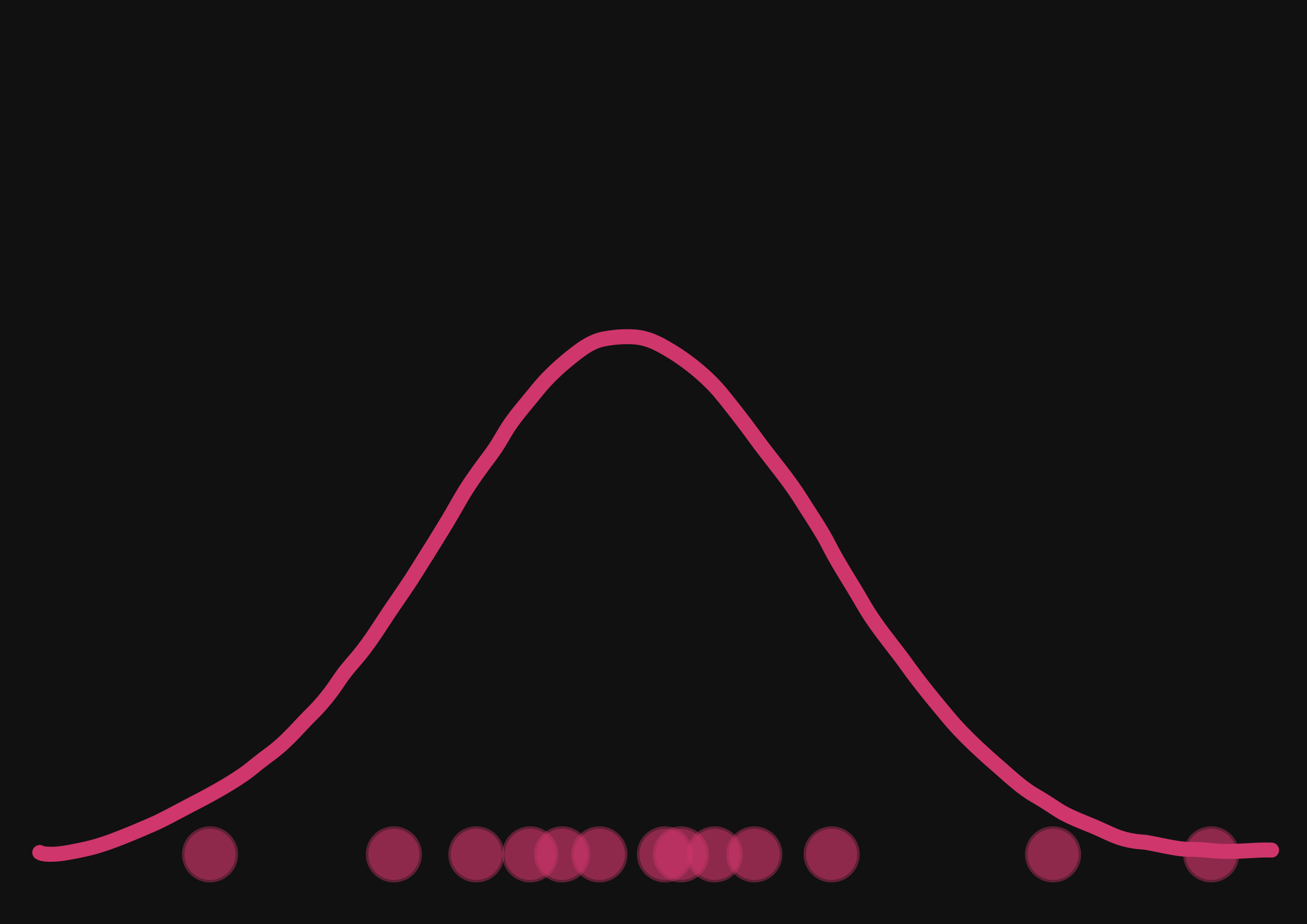
With a few simulations it's hard to approximate the distribution.
$\to$ we need more simulations
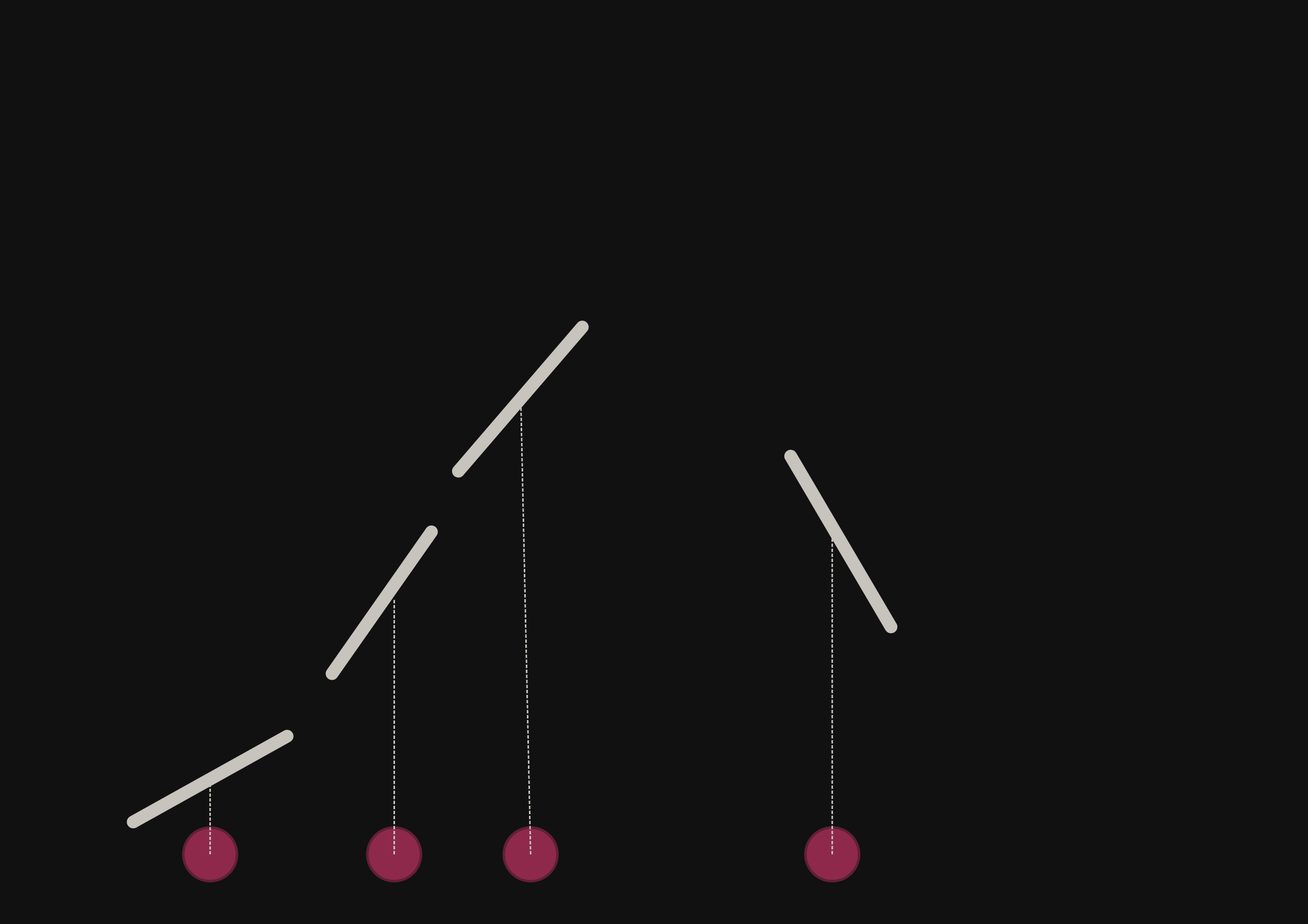
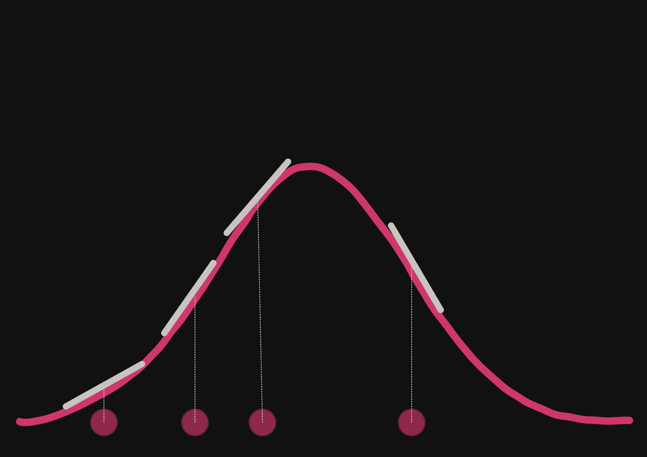
but if we have a few simulations
and the gradients
then it's possible to have an idea of the shape of the distribution.
Proof on concept on a toy model: Lotka Volterra
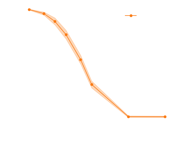

- Yes! Adding the gradients speeds up the convergence.
- Ongoing work $\to$ apply it to our cosmological simulator.